Finding the best fit rotational broadening and radial velocity

[NOTE] For this tutorial, you’ll need to have our sibling package muler installed, which can be done with pip install muler.

A common occurrence in astronomy is when we have a data spectrum and we want to find the best fit \(v\sin(i)\) and \(v_r\).

In this demo we will show some simple ways to use gollum to find the model with the best fit rotational broadening and radial velocity, assuming a fixed template.

import astropy.units as u
import matplotlib.pyplot as plt
import numpy as np

from gollum.phoenix import PHOENIXSpectrum
from muler.hpf import HPFSpectrumList
from tqdm.notebook import tqdm

%config InlineBackend.figure_format='retina'

For this demo we will need some real world example data

Let’s use data of an A0V star from HPF.

You can get free example data from the muler_example_data GitHub repo.

The example data is preloaded into gollum’s repo; it was downloaded from this link.

raw_data = HPFSpectrumList.read('../tutorial_data/Goldilocks_20210517T054403_v1.0_0060.spectra.fits')

# Clean the data with a series of post-processing steps
full_data = raw_data.sky_subtract().deblaze().trim_edges((4, 2042)).normalize().stitch()

As a final step, we will mask the telluric absorption lines. This step can sometimes benefit from hand-tuning.

data = full_data.mask_tellurics(threshold=0.999, dilation=13)

We will restrict our fits to the region with the highest density of H lines.

data = data[8500*u.AA:8950*u.AA]
data = data.normalize()

ax = data.plot(marker='.', linestyle='None')
ax.set_xlim(8500, 8950)
plt.show()

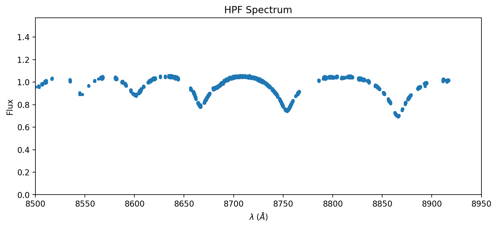
OK, that’s our data spectrum against which we will compare models. You can see large voids in the spectrum due to our telluric masking– that’s fine, the data need not be contiguous or evenly sampled to estimate a best fit model. We will resample the model to the data.

We can choose 3 dimensions in our grid: \(T_{\mathrm{eff}}, \log(g), \left[\mathrm{Fe}/\mathrm{H}\right]\)

template = PHOENIXSpectrum(teff=9600, logg=4.5, Z=0, download=True)

We then want to rotationally broaden and RV shift the spectrum. We’ll guess the \(v\sin(i)\) and \(v_r\) values to be 150 km/s and -50 km/s, respectively:

spec = template.rotationally_broaden(150).rv_shift(-50).instrumental_broaden(55000).resample(data).normalize()

ax = data.plot(label='Data')
spec.plot(ax=ax, label='Doctored Model')
ax.legend()
plt.show()

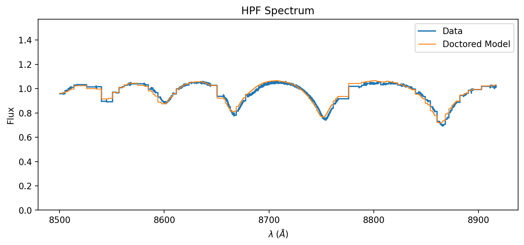
You can see that our guesses are off. Let’s do a grid search for \(v\sin(i)\) and \(v_r\).

vsinis = np.linspace(1, 150, 20)
rvs = np.linspace(-100, 100, 20)
search_vsini, search_rv = np.meshgrid(vsinis, rvs, indexing='ij')

We will compute the RSS (Residual Sum-of-Squares) loss for each value of \(v\sin(i)\) and \(v_r\).

@np.vectorize
def rss(vsini, rv):
    model = template.rotationally_broaden(vsini).rv_shift(rv).instrumental_broaden(55000).resample(data).normalize()
    return np.sum((data.flux - model.flux)**2)

loss = rss(search_vsini, search_rv)

best_i, best_j = np.unravel_index(np.argmin(loss), (20, 20))
best_vsini, best_rv = vsinis[best_i], rvs[best_j]
best_vsini, best_rv

(102.94736842105263, 15.789473684210535)

plt.imshow(loss, extent=[rvs.min(), rvs.max(), vsinis.min(), vsinis.max()], aspect='auto', origin='lower', interpolation='gaussian')
plt.scatter(best_rv, best_vsini,  marker='*', c='w', ec='k', s=200)
plt.colorbar(label='RSS')
plt.xlabel(r'$v_r \quad [\mathrm{km}/\mathrm{s}]$')
plt.ylabel(r'$v\sin(i) \quad [\mathrm{km}/\mathrm{s}]$')
plt.show()

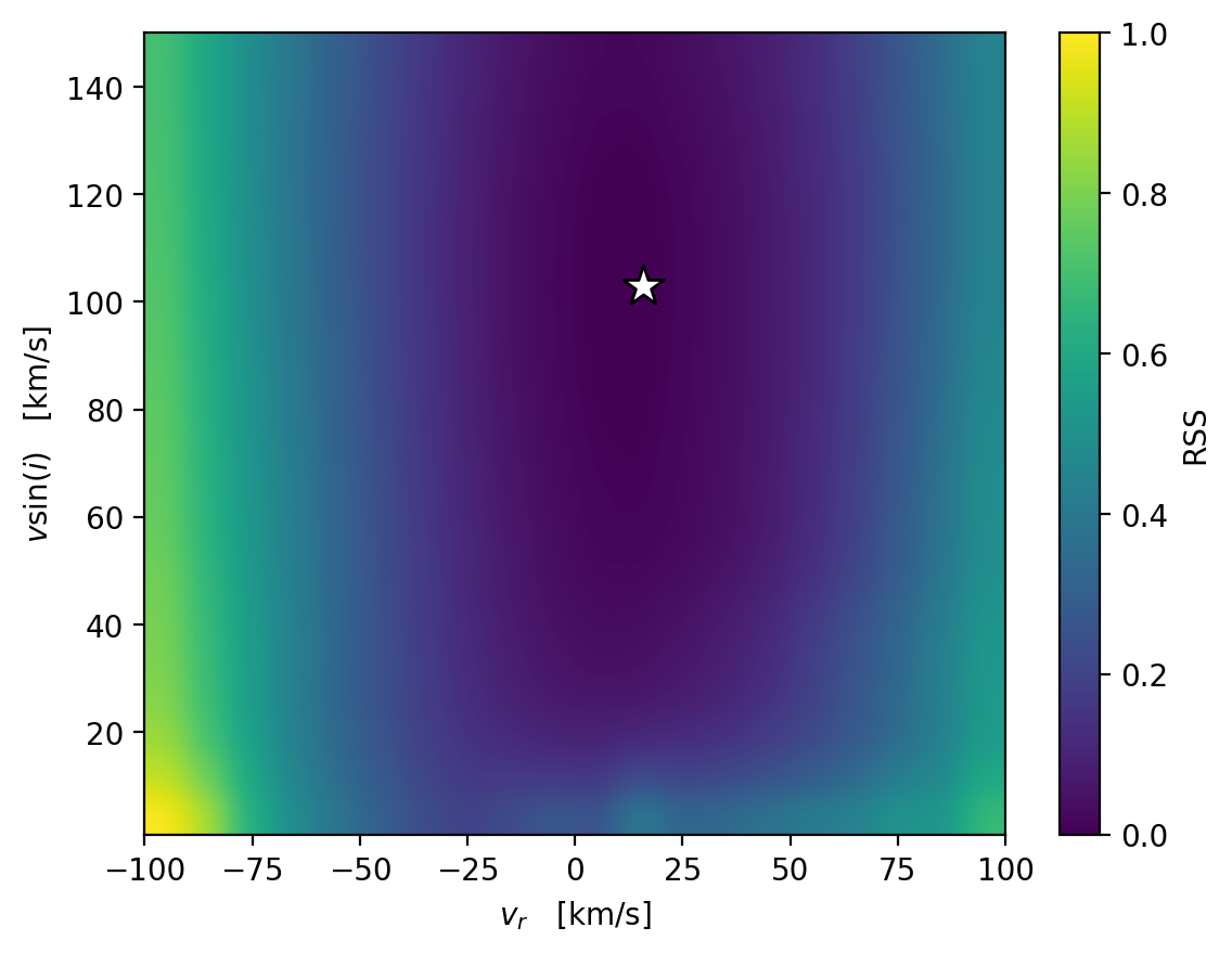
Awesome, we have found the \(v\sin{i}\) and \(v_r\) with the closest match to the data.

best_spec_full = template.rotationally_broaden(best_vsini).rv_shift(best_rv).instrumental_broaden(resolving_power=55000)
best_spec = best_spec_full[data.wavelength.min():data.wavelength.max()].normalize()

How does the best fit look by-eye?

ax = (data/data.flux.max()).plot(marker='.', linestyle='None')
(best_spec/best_spec.flux.max()).plot(ax=ax)
ax.set_title(rf'$v\sin(i)$ = {best_vsini:0.0f} km/s, $v_r$ = {best_rv:0.1f} km/s')
plt.show()

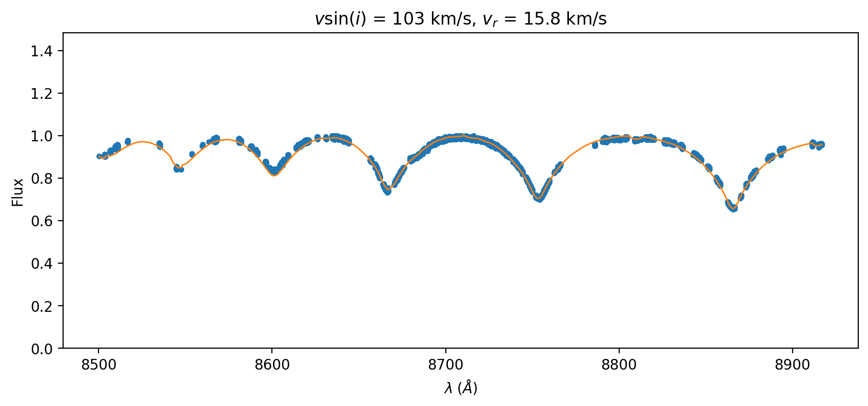
Excellent! That’s much better than our initial guess.